Privacy Policy

Privacy Policy for demand-curve.blogspot.com

If you require any more information or have any questions about our privacy policy, please feel free to contact us by email at topgear832@gmail.com.

At demand-curve.blogspot.com, the privacy of our visitors is of extreme importance to us. This privacy policy document outlines the types of personal information is received and collected by demand-curve.blogspot.com and how it is used.

Log Files
Like many other Web sites, demand-curve.blogspot.com makes use of log files. The information inside the log files includes internet protocol ( IP ) addresses, type of browser, Internet Service Provider ( ISP ), date/time stamp, referring/exit pages, and number of clicks to analyze trends, administer the site, track user’s movement around the site, and gather demographic information. IP addresses, and other such information are not linked to any information that is personally identifiable.

Cookies and Web Beacons
demand-curve.blogspot.com does use cookies to store information about visitors preferences, record user-specific information on which pages the user access or visit, customize Web page content based on visitors browser type or other information that the visitor sends via their browser.

DoubleClick DART Cookie
.:: Google, as a third party vendor, uses cookies to serve ads on demand-curve.blogspot.com.
.:: Google's use of the DART cookie enables it to serve ads to users based on their visit to demand-curve.blogspot.com and other sites on the Internet.
.:: Users may opt out of the use of the DART cookie by visiting the Google ad and content network privacy policy at the following URL - http://www.google.com/privacy_ads.html

Some of our advertising partners may use cookies and web beacons on our site. Our advertising partners include ....
Google Adsense


These third-party ad servers or ad networks use technology to the advertisements and links that appear on demand-curve.blogspot.com send directly to your browsers. They automatically receive your IP address when this occurs. Other technologies ( such as cookies, JavaScript, or Web Beacons ) may also be used by the third-party ad networks to measure the effectiveness of their advertisements and / or to personalize the advertising content that you see.

demand-curve.blogspot.com has no access to or control over these cookies that are used by third-party advertisers.

You should consult the respective privacy policies of these third-party ad servers for more detailed information on their practices as well as for instructions about how to opt-out of certain practices. demand-curve.blogspot.com's privacy policy does not apply to, and we cannot control the activities of, such other advertisers or web sites.

If you wish to disable cookies, you may do so through your individual browser options. More detailed information about cookie management with specific web browsers can be found at the browsers' respective websites.

How the Demand Curve is Consistent with the Quantity Theory of Money

The AD curve is consistent with the quantity theory of money.

The expansino shifts the AD schedule from AD to AD1. I nthe very short run, if the price level were to remain at the Po, the economy would move to point E1. This would cause excess demand in the goods and labour markets, which would in turn force up wages and prices.
The classical model assumes instance adjustment, the economy would go directly to point E2, with no charges in output, and a higher price level. In the long run, quantity theory of money holds.

If you were interested in this post then visit the 'how to derive the aggregate demand curve' post for related material.

Supply, Demand and Equilibrium Price

Supply, Demand and Equilibrium Price

According to conventional economic theory market price is fixed by the following mechanism:

• Demand. The demand curve D illustrates the variation of a demand Q in relation to the variation of a price P. This function is characterized by an inversely proportional curve where demand drops when the price goes up (and vice-versa). If the price of a good or service is too high (P1), the demand drops (Q1) while in the opposite situation (low price; P2) demand grows (Q2).
• Supply. The supply curve S illustrates a variation of supply according to a variation of price P. This function is characterized by a directly proportional curve where supply increases as the price goes up. Supply grows (Q1 to Q2) when the price increases (P1 to P2) since profits would be higher.
• Equilibrium Price. The intersection of the demand curve D and the supply curve S represents the equilibrium price Pe where a quantity Qe of goods will be sold. Changes in the market (moving curves D or S to the left or the right) will change the equilibrium price.

Supply and Demand of Government qua Natural Monopoly

In an earlier post, I described a scalar model of consent. I here use that model to analyze the supply and demand of government services. Specifically, I explore the origin and development of government qua natural monopoly. I plan in a later post to apply a similar analysis to government qua provider of public goods.

A government that enjoys a natural monopoly on satisfying the express demand for its services will have the power, and incentive, to expand to meet non-express demand. The result: a supply of more government services, at a higher price, than citizens in fact want. In an extreme case, satisfying the implied or hypothetical demand for government services may result in an oversupply so gross that consumers expressly assign it a negative price. In other words, consumers of government services may actually object to what they supposedlywant.

Government represents a sort of service industry, albeit one marked by some peculiar features. For one thing, governments can often lay plausible claim to qualifying as natural monopolies. (Perhaps that is not so peculiar; David Friedman convincingly argues that natural monopolies pervade sufficiently small markets.) Figure 1, below, offers a fairly conventional graph of the economic features of government qua natural monopoly.





(In figure 1, "MC" stands for "marginal costs of production"; "ATC" for "average total costs of production"; and "D" for "aggregate demand." Because we here portray a monopoly aggregate demand equates to "AR," or "average revenue." The various uses of "P" mark prices; "Q" of quantities. The lowercase "m," as in "Pm," designates the monopoly price. "Qm" of course corresponds to the monopoly quantity. In like fashion, "r" designates the regulated price and quantity, and "c" the competitive ones.)

So it goes, at least, in the standard economic view, which concerns only expressly consensual transactions. But as I noted earlier,, we might do well to also consider transactions marked by less than express consent. Government monopolies, for instance, typically claim to respond to implied and hypothetical consent. What does a market based on non-express consent look like? Figure 2, below, illustrates.





Figure 2 shows the non-express demand, marginal revenue, monopoly price, and monopoly supply of government services. All those non-express measures come marked with "(n)" suffixes. The express measures from figure 1 remain, but now carry "(e)" suffixes to distinguish them from the newly added material. (For the sake of clarity, I've dropped from figure 2 some of the information offered in figure 1.)

Figure 2 illustrates three interesting results. First, non-express demand, because it includes transactions beyond those expressly agreed to, traces a curve to the right of typical (i.e., express) demand. Second, due to its speculative nature, non-express demand of necessity charts a somewhat more fuzzy line than express demand does. Figure 2 thus draws the non-express demand and marginal revenue curves as relatively imprecise blobs.

Third, and most crucially, figure 2 illustrates that a government monopoly meeting non-express demand may provide more services, at a higher price, than consumers in fact demand. How can government agents get away with thereby supplying and getting paid for grossly inefficient level of services? Recall that we charitably but reasonably supposed that in a market based on expressly consensual transactions, government will enjoy a natural monopoly. Government agents can thereby lay claim to a monopoly on the initiation of coercion. They can all too easily wield that power to expand their market share, claiming a mandate to satisfy implied or hypothetical consent. And, given the super-monopoly profits thereby afforded, they have powerful incentives to do so.

Figure 2 only hints at something that figure 3, below, makes explicit: Government based on non-express consent may supply—"oversupply," really—a level of service that consumers expressly value at less than zero. That result follows quite directly from the simple, if somewhat unusual, expedient of following the express demand curve even as it plunges below the x-axis. Economists do not generally explore that region of "negative demand," granted, but they seldom have reason to do so. Figure 3, because it tracks both express and non-express transactions, gives us good reason to spell out what happens when a supposedly justified supply meets actual consumer demand.





What, in sum, does this application of "consent theory" (as I style it) teach? Government services, because they have power and incentives to expand from natural monopolies based on express consent to coercive monopolies based on implied or hypothetical consent, threaten to provide more government than consumers really want. In some cases, consumers may afford negative value to the resulting oversupply of government services. We thus might say that figure 3 illustrates, in the iconography of economics, the causes and effects of tyranny.

That paints a rather grim—but, I would argue, accurate—picture of how government can grow from a natural monopoly into an artificial, and unwelcome, one. Note, however, that I have not yet invoked the public goods justification for government power. I'll take that up my next post on consent theory, explaining why a government that aims to meet the hypothetical demand for public goods runs a reduced risk of supplying services to which that consumers assign negative value. In other words, governments based on the hypothetical demand for public goods tend to become bloated but not monstrous.

Business Revenues

The meaning of revenue

Revenue (or turnover) is the income generated from the sale of output in product markets. There are two main revenue concepts to grasp at this stage:

• Average Revenue (AR) = Price per unit = total revenue / output
• Marginal Revenue (MR) = the change in revenue from selling one extra unit of output

The table below shows the demand for a product where demand varies inversely with the price.

Price per unit (average revenue)	Quantity Demanded (Qd)	Total Revenue (TR)	Marginal Revenue (MR)
£s	units	£s	£s
400	220	88000
370	340	125800	315
340	460	156400	255
310	580	179800	195
280	700	196000	135
250	820	205000	75
220	940	206800	15
190	1060	201400	-45

Average and marginal revenue – the important relationships

In our example in the table above, as price per unit falls, demand expands and so too does total revenue, although because the demand curve is downward sloping, the average revenue falls as more units are sold. This causes marginal revenue to decline. Eventually once marginal revenue becomes negative, a further fall in price (e.g. from £220 to £190) causes total revenue to fall.

Because the price per unit is declining, total revenue is rising at a decreasing rate and will eventually reach a maximum (see the next paragraph).

Elasticity of demand and total revenue

When a firm faces a perfectly elastic demand curve, then average revenue = marginal revenue (i.e. extra units of output can all be sold at the ruling market price). However, most businesses face a downward sloping demand curve! And because the price per unit must be cut to sell extra units, therefore MR lies below AR. In fact he MR curve will fall at twice the rate of the AR curve. You don’t have to prove this for the exams – but it is worth remembering that the marginal revenue curve has twice the slope of the AR curve!

The total revenue for any business is maximised when marginal revenue (MR) = zero. Once MR becomes negative, total revenue falls if extra units are sold. This is shown in the next diagram.

Total revenue is shown by the area underneath the firm’s demand curve (average revenue curve).

COMPETITION AND THE SEARCH FOR AN HONEST BUCK

Instructional Goals: You will understand:

• How to measure consumers' surplus and deadweight loss.
• What a residual demand curve is and how to use one.
• The importance of property rights for exchange to take place; the nature of externalities or spillovers, and the Coase theorem.
• The difference between a buyer and a seller.

Lecture 2:30 PM to 4:00

Consumption is the purpose of all economic activity. Work is economically meaningful only if it produces something of value to someone -- that is, only if there is a consumer out there who wants to buy it. What is true of the economy as a whole, is equally true for the organizations that comprise it. This principle is not a call to hedonistic self indulgence. Putting the customer first is a discipline competition imposes upon producers. You can work as hard as you want, but unless you're creating more value than you are expending, you are wasting your resources and will eventually be put out of business. It is this discipline that drives producers to create more and more value for less and less effort -- in other words, make us richer.

Increasing competition tightens the screws of market discipline -- benefiting consumers, but making it harder for organizations to earn an honest buck, i.e., more than normal returns on one's investment.

Under perfect competition YOU cannot earn more than a normal return on your investment. So what are the characteristics of perfect competition?

• Perfectly homogeneous goods. All organizations supplying the market sell an identical product or, at the very least, consumers view their products as identical and are indifferent between them. A corollary of this characteristic is: Perfect divisibility of output.
• Perfect information. Producers and consumers, buyers and sellers, have all relevant information about all prices, costs, and quality of all products. A corollary of this characteristic is: No transaction costs. Buyers and sellers do not encounter search, bargaining/negotiation, enforcement or monitoring costs; delivery is free and occurs precisely when needed. Another corollary is: No externalities or spillover costs and benefits that are not captured by the parties to the exchange.
• Price taking. Buyers and sellers cannot individually influence the price at which products can be purchased or sold. The corollary of this characteristic is: Free entry and exit, that is, organizations can enter or exit a market without incurring a cost.

Obviously, you will want to earn the highest possible return on your investment. The only way to do so is to change markets so these conditions do not obtain (e.g., consumer indifference) or take advantage of situations where they cannot (e.g., perfect information).

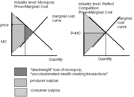
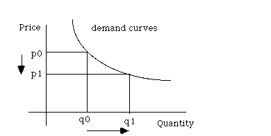
As you learned in economics, a demand schedule reflects willingness and ability to pay and a supply schedule, willingness and ability to sell. The sum of the difference between what customers were willing to pay and the price paid represents the exchange value provided by a product. It is called a consumer surplus and is measured by the area under the demand schedule and above the price line. Conversely, the area above the supply schedule and below the price line is the producer surplus.

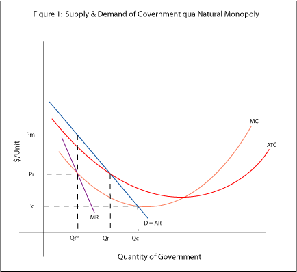
An unconstrained profit-maximizing monopoly, producing a perfectly homogeneous product and charging a single price, would set output and price to equate marginal revenue with marginal cost, resulting in a substantial deadweight loss.

The following figure shows the case of a revenue (not profit) maximizing natural monopoly. A revenue maximizing entity operates where marginal revenue is zero. A so-called natural monopoly is one in which average total cost (ATC) decreases at a decreasing rate throughout the relevant range of output. This is so in the instance shown below because marginal cost is constant, while large capacity (or fixed) costs are spread over total output. Under these conditions, where a single price is charged for each unit of output, the consequent deadweight loss is substantial.

Natural monopolies are not necessarily inefficient -- although lack of competion encourages sloth and other bad things. Given perfect information, consumers could band together and bribe the potential monopolist to offer the optimal quantity of of the good or service in question.

Elasticities and the Residual Demand Curve

This course makes repeated use of two related concepts to analyze both price competitive and noncompetitive industries: (1) price elasticity of demand or supply and (2) the demand curve facing a single organization's product or service: the residual demand curve. The price elasticity of supply or demand aids in understanding how an industry is likely to respond to changes in demand or supply. The residual demand facing a single organization allows you to understand and exploit the demand for your service and products. The following discussion explains how the elasticity of the residual demand curve is related to the assumption that a price competitive organization cannot affect price.

Elasticities of Demand and Supply

If either the demand or supply curve shifts, the competitive equilibrium changes, and the shapes of the demand and supply curves influence how the new equilibrium compares to the old. For example, if the demand curve is perfectly flat, the competitive price remains unchanged, even if the supply curve shifts radically.

One concept used to characterize the shape of demand or supply curves is the price elasticity of demand or supply (often the word price is omitted). The price elasticity of demand at price p and quantity Q is approximately the percentage change in quantity divided by the percentage change in price (ÆQ/Q) ÷ Æp/p) = (p/Q) (ÆQ/Æp).

Because the elasticity is the ratio of two percentage terms, the elasticity is invariant to changes in scale of either price or quantity (it is a pure number without scale itself). For example, if price is measured in cents rather than dollars, the elasticity is unchanged even though the slope of the demand curve, ÆQ/Æp, does change. The technical definition of the price elasticity is (p/Q)(dQ/dp). Similarly, the elasticity of supply is (approximately) the percentage change in quantity supplied in response to a 1 percent change in price. The elasticity of demand is a negative number, and the elasticity of supply is usually, but not always, positive.

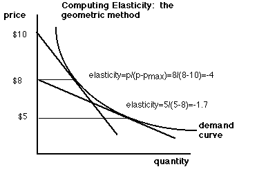
If a 1 percent increase in price leads to a more than a 1 percent reduction in the quantity demanded (so that the total amount paid in the market falls) a demand curve is called elastic. That is, an elastic demand curve has an absolute value of the elasticity of demand greater than one (the absolute values of 1 and -1 are both 1). It is common to omit the phrase the absolute value of when discussing the price elasticity of demand. The statement, "The price elasticity of demand is 2," is interpreted to mean that the price elasticity is -2.

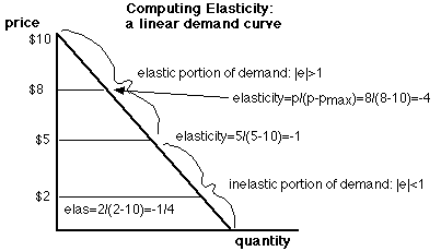
When the absolute value of the elasticity of demand is 1, the demand curve is of unitary elasticity. In that case, a 1 percent change in price causes a 1 percent change in the quantity demanded, and the total amount paid (total revenues) remains constant. If the absolute value of the elasticity of demand is less than 1, the demand curve is inelastic; a 1 percent increase in price causes less than a 1 percent decline in the quantity demanded, and the total amount paid rises.

In general, the elasticities of demand and supply depend upon many economic factors, such as the level of output, the availability of substitute products, and the ease with which suppliers can alter production. For example, as more substitute products are available, consumers find it easier to substitute for a product if its price rises, which makes its demand curve more elastic. Similarly, the more flexible the production process of a organization, the more likely it is that the organization can greatly increase production in response to a price increase, which tends to increase the elasticity of supply.

Price Taking Among Price competitive Organizations and the Residual Demand Curve

Price competitive organizations are often described as price takers; they believe that they cannot affect the market price and must accept, or take, it as given. There are three equivalent ways to state this result, all of which are used in this course:

• A price competitive organization is a price taker.

• The demand curve facing a price competitive organization is horizontal at the market price.

• The elasticity of demand facing a price competitive organization is infinite.

A organization is a price-taker if it faces a horizontal demand curve, because a horizontal demand curve has an infinite price elasticity of demand. If a organization facing an infinite price elasticity raises its price even slightly, it loses all its sales. Alternatively stated, by lowering its quantity, the organization cannot cause the price to rise. In contrast, a organization facing a downward-sloping demand curve can raise its price by decreasing its output.

If the number of organizations in an industry (an industry is made up of all the organizations supplying products or services with identical attributes) is large, the demand curve facing any one of them is nearly horizontal (elasticity of demand is infinite) even though the demand curve facing the industry is downward sloping (elasticity is relatively small). Indeed, for most market demand curves, there do not have to be very many organizations in an industry for the elasticity of demand facing a particular organization to be large.

To show this result, it is necessary to determine the demand curve facing a particular organization: the residual demand curve. A organization sells to people whose demands are not met by the other organizations in the industry. For positive quantities of residual demand, the residual demand, D,(p), is the market demand, D(p), minus the supply of other organizations, S_o(p):

D_r(p) = D(p) - S_o(p)

If S_o(p) is greater than D(p), D_r(p) is zero.

Figure 4.6b shows the market demand curve and the supply of all the organizations except one. The horizontal difference between the market demand curve and the supply of the other organizations is the residual demand facing a particular organization, Figure 4.6a. The horizontal difference is the quantity demanded by the market at a given price minus the supply of other organizations at that price.

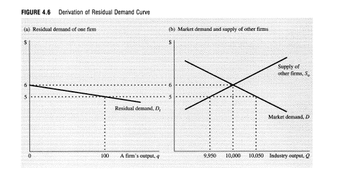
For example, in Figure 4.6b, at a price of $5, market demand is 10,050 units and the supply of the other organizations is 9,950 units. That is, the other organizations are not willing to meet the entire market demand at $5; the difference between demand and the supply of other organizations is 100 units. Thus, at $5, the organization's residual demand is 100 units. At $6, the supply of other organizations equals the market demand. The residual demand facing the organization in Figure 4.6a is zero. Were price to rise even higher, other organizations would be willing to supply even more than is demanded. Thus, at any price greater than or equal to $6, the organization in Figure 4.6a sells no units.

The residual demand curve facing the organization, Figure 4.6a, is much flatter than the market demand curve, Figure 4.6b. Similarly, the single organization's demand elasticity is much higher than the market elasticity. As drawn, the elasticity of demand for the individual organization, from $5 to $6, is -11, whereas the corresponding market arc elasticity of demand is -0.025. In other words, the organization's residual demand elasticity is 440 times as elastic as the market elasticity.

More generally, if there are n identical organizations in the industry, then the elasticity of demand facing any one organization i is

e _i = e n - h _o n /(n - 1),

where e is the market elasticity of demand (a negative number), h _o is the elasticity of supply of the other organizations (a positive number), and (n -1) is the number of other organizations.

Thus for a given market elasticity, as the number of organizations in an industry, n, increases, the elasticity facing a single organization i, e _i grows large in absolute value (more negative). Similarly, the larger the elasticity of supply of the other organizations,

or the more of these other organizations, the larger in absolute value (more negative) is the elasticity of demand facing organization i.

Table 4. 1 shows how the elasticity of demand facing a single organization varies with the number of organizations and the market elasticities, given that the elasticity of supply of other organizations is completely inelastic (h _o = 0). For example, if the market elasticity is unitary (e = 1) and there are 50 organizations, then e _i = -50. That is, if a organization were to increase its price by 1 percent, the quantity it sells would fall by about 50 percent. If there are 1000 organizations, e _i = -500, so that if the organization were to raise its price by a tenth of a percent, the quantity it sells would fall by 50 percent. Thus, even if the market elasticity is completely inelastic, if there are a large number of organizations in the industry, the elasticity of demand facing a single organization is very large (see Example 4.2).

EXERCISES

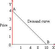
1. Please draw figure so that the inverse demand schedule is Q = 100 - p (both the vertical and horizontal intercepts are at 100). Note that at p = 100, Q = 0; at p = 0, Q = 100; and at p = 50, q = 50.

2. Please draw figure so that the inverse supply schedule is Q = p. Note that at p = 100, Q = 100; at p = 0, Q = 0; and at p = $50, q = 50.

3. Find the competitive equilibrium price and quantity (set Q = p, 100 - p = p, 100 = 2p, p = ?, q = ?

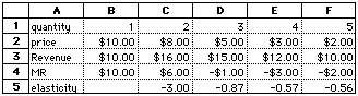
4. Calculate total revenue (TR) = pQ =

5. Calculate consumers' surplus (100 - p)Q/2 =

6. Calculate producers' surplus pQ - C, where C = pQ/2 =

7. Draw identical figure to thone described in steps 1 & 2, but include marginal revenue schedule (MR) with the following equation Q = 50 - .5p

8. Calculate profit maximizing output (set Q = MR, 50 - .5p = p, 50 = 1.5p, Q = ).

9. Use the inverse demand schedule (Q = 100 - p) to calculate the profit maximizing price (set p = 100 - 33.33, p =

10. Calculate total revenue (TR) = pQ =

11. Calculate consumers' surplus (100 - p)Q/2 =

12. Calculate producers' surplus pQ - C, where C = pQ/2 =

13. Show calculation for deadweight loss D = $33.33 (16.67)/2 =

13. Calculate Price Elasticity, where p = $50, Q = 50, Price Elasticity = |?|; p = $75, Q = 25, Price Elasticity = |?|; p = $25, Q = 75, Price Elasticity = |?|

14. Calculate Price Elasticity, where p = $66.67, Q = 33.33, Price Elasticity = |?|

15. Using the inverse elasticity rule (Ramsey optimal pricing): p-mc/p = 1/|Price Elasticity| = calculate the optimal markup where Price Elasticity is |2| and marginal cost is $33.33

EXAMPLE 1

Assume a price competitive industry with free entry and exit. What would happen to industry output, optimal organizational scale (assuming all organizations had access to identically the same technologies), and the equilibrium price, if government imposed a fixed fee per year on each organization participating in the industry?

___________

Answer: The following figure shows that, starting from long-run normal-profit equilibrium, an increase in fixed costs raises average costs from AC₁ to AC₂. At the original price each organization would lose money, so some organizations would exit the industry (the number of organizations goes from n₁ to n₂). Remaining firms produce more than before (q₁ instead of q₂). Total output falls from Q₁ = nq₁ to Q₂ = nq₂. Price rises to P₂.

Demand Schedule, Function and Law

D(demand) qd	Schedule P
10	0
8	1
4	2
1	3
0	4

(A) Demand Schedule : The various quantities demanded of a particular commodity are presented here in a schedule. At arbitrarily chosen prices, the quantity of a commodity an individual consumer is expected to demand, is explained by the schedule. Since quantity demanded (q_d) depends on the relevant prices of goods, the two can be expressed in the form of an algebraic function as well. The schedule shows that as price goes on rising (from zero to 4) the quantity demanded goes on falling (from 10 to zero).

The scheduled information has been presented in the form of a demand curve in Figure 2 (below). In the figure, the units of quantity of the goods have been measured along the horizontal axis (OX) and the respective prices have been shown along the vertical axis (OY). The curve intersects OY axis at point A which shows highest price at which quantity demanded is zero. On the contrary the curve intersects OX axis at point B showing largest quantity demanded where price is zero. Both OA and OB are said to be intercept quantities when one of the variables assumes zero value. Note that demand curve is sloping downward. This follows the law of demand (given below). But the demand curve of such a shape is obvious from the fact that quantities demanded and price in the demand schedule hold an inverse relationship.

Quantity Demanded q_d
Figure 2

(B) Demand Function: The price-demand relationship shown above can be expressed in the form of a demand function as follows:

q_d = 10 - 3P

On substitution of any scheduled value of P we get the relevant value of the quantity demanded. Thus when P = 1 then q_d =10 - 3 (1) = 7 or when P = 3, then q_d = 10 - 3 (3) = 1 etc.

(C) Law of demand: The law of demand explains the inverse relation between quantity and price in general. It can be stated as follows:

"Ceteris Paribus (other things remaining equal), the quantity of a good demanded will rise (expand) with every fall in its price and the quantity of a good demanded will fall (contract) with every rise in its price."

In a functional form this can be stated as,

q_d = f (P) [ Y, Ps, N, Z ]_const.

This explains that q_d, the quantity of a good demanded functionally depends on its price P. However, the quantity demanded is also causally related to other factors such as income of an individual (Y), prices of substitutes (Ps), number of members in the family (N) and the tastes of the consumer (Z). In order to satisfy price-demand relation, the effect of these other variables has been restrained by assuming them to be constant.

Initially, the law of demand was based on the principle of diminishing marginal utility (DMU). But in that case it was implied that utility is cardinally or absolutely measurable. There were other practical difficulties in the DMU approach as well. Therefore recently attempts have been made to place the law of demand on the empirical and realistic basis. One such attempt is in the form of Indifference Curve (IC) analysis. Under the IC approach it is enough to measure utility in ordinal or relative terms.

(D) Rise or Fall and Increase or Decrease in demand: On a given demand curve as we move downwards from point A in the direction of B, the quantity demanded goes on rising with every successive fall in price. On the contrary, moving from point B to A shows a fall in the quantity demanded with every successive rise in the price. Marshall has called this process rise and fall or expansion and contraction in the demand. Therefore, in this case the price of the quantity (and the change in it) plays an important part. Here, a change in the quantity demanded is indicated with movement along the demand curve (up or down accordingly). This change is subject to the ceteris paribus condition.

On the other hand, other factors are also likely to alter the quantity demanded. This can be expressed by a shift in the curve. Such an upward shift in the demand curve (Figure 3) has been shown by a new and higher demand curve (A₁B₁) in the figure.

Figure 3

At a given price OP on the original demand curve (AB), the quantity demanded is Oq but on the new demand curve (A₁B₁) it has increased to Oq1. On the other hand, if we begin with the A₁B₁ demand curve as the initial demand curve and consider demand to have reduced (to AB) then the quantity demanded reduces from Oq1 to Oq. Such a change in the demand, arising out of a shift in the demand curve is known as an increase (if it is towards the right of the original demand curve) and a decrease (if it is towards the left of the original demand curve) in the demand, respectively.

The demand curve may shift and quantity demanded may increase or decrease, due to changes in a number of factors (apart from price), say the income (Y) of a consumer (when he becomes richer or poorer). A similar effect can be noticed with a rise or fall in the price of substitute (Ps) goods. For instance, tea and coffee or soaps of different brands are substitutes of each other. Therefore a rise in price of pasta may result in a reduction in the consumption of pasta and simultaneously an increase in the consumption of bread to that extent and vice versa. Or the demand curve may shift and quantity demanded may increase at the old price if there is a sudden increase in the number of members in a family (N), (say because of the unexpected arrival of guests). Finally, a shift in the demand curve may also be the result of the change in the tastes of a consumer. A cigarette or liquor consumer may become addicted because of which his demand for such goods will rise remarkably even at the old price.

There is an important difference between the change in the quantity demanded of a particular commodity and change in the demand for that commodity. While the former is influenced by the single factor: price, the latter is influenced by various other factors apart from price. A change in the quantity demanded is represented by a movement along the demand curve, while a change in the demand is represented by a shift of the curve (towards the left in case of a decrease and towards the right in case of an increase).